Beyond 2.5D: A Review of Non-Planar Slicing Algorithms and Principal Stress Alignment in Robotic Continuous Fiber Printing

January 2025 40 min read

Vector-Field Based Toolpath Generation for Multi-Axis Composite Additive Manufacturing

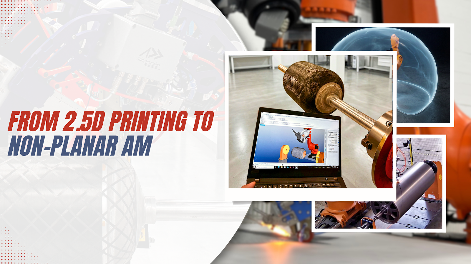
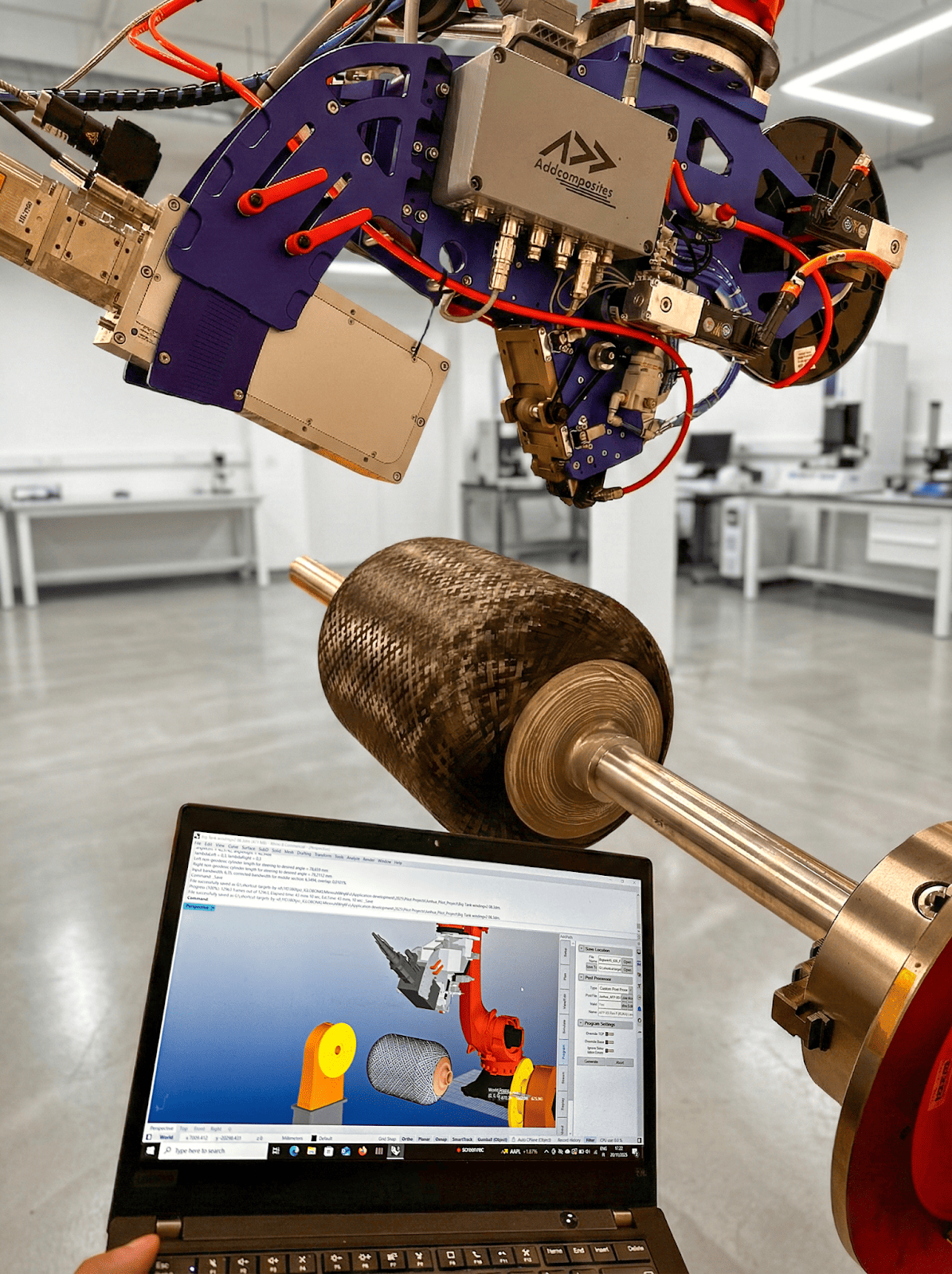
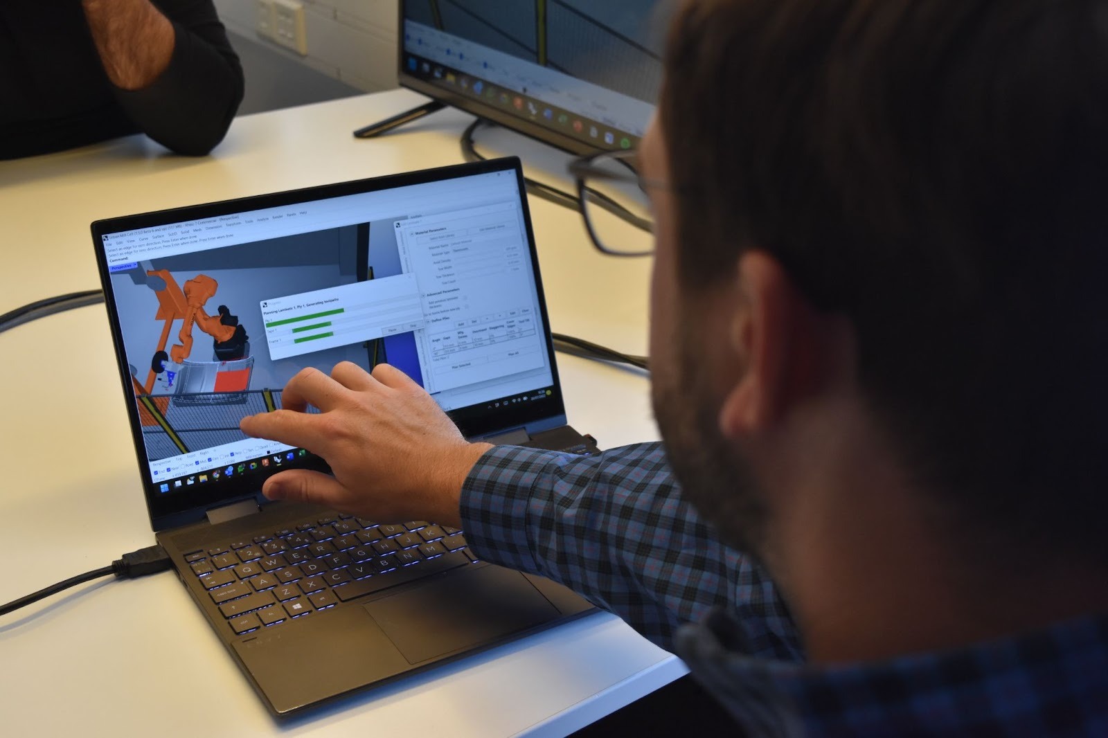
FIGURE 1: Hero Image — Stress-Aligned Continuous Fiber Printing on Curved Surface

Principal Stress-Guided Spatial Fiber Printing

6-DOF robotic deposition of continuous fiber along σ₁ directions on non-planar toolpaths

Deposited Fiber Tows

σ₁ Principal Stress Direction

Part Surface (Non-Planar)

Continuous Fiber Non-Planar Toolpath FEA-Driven Placement Load-Path Optimised

Concept based on Fang et al. (2024) — "Toolpath Generation for High Density Spatial Fiber Printing Guided by Principal Stresses" — arXiv:2410.16851

Introduction

The vast majority of additive manufacturing systems—from desktop FDM printers to industrial fiber placement robots—operate under a fundamental constraint: they slice parts into flat, horizontal layers and deposit material in a plane-by-plane fashion. This "2.5D" paradigm works well for prismatic geometries but introduces significant limitations when manufacturing parts with curved surfaces, complex load paths, or where fiber orientation directly determines structural performance.

For continuous fiber reinforced composites, this limitation is particularly consequential. The mechanical properties of a carbon fiber composite are highly anisotropic: tensile strength and stiffness along the fiber axis can exceed transverse properties by an order of magnitude. When fibers are constrained to planar layers, they cannot follow the three-dimensional stress trajectories that actual loads create—resulting in suboptimal structural efficiency.

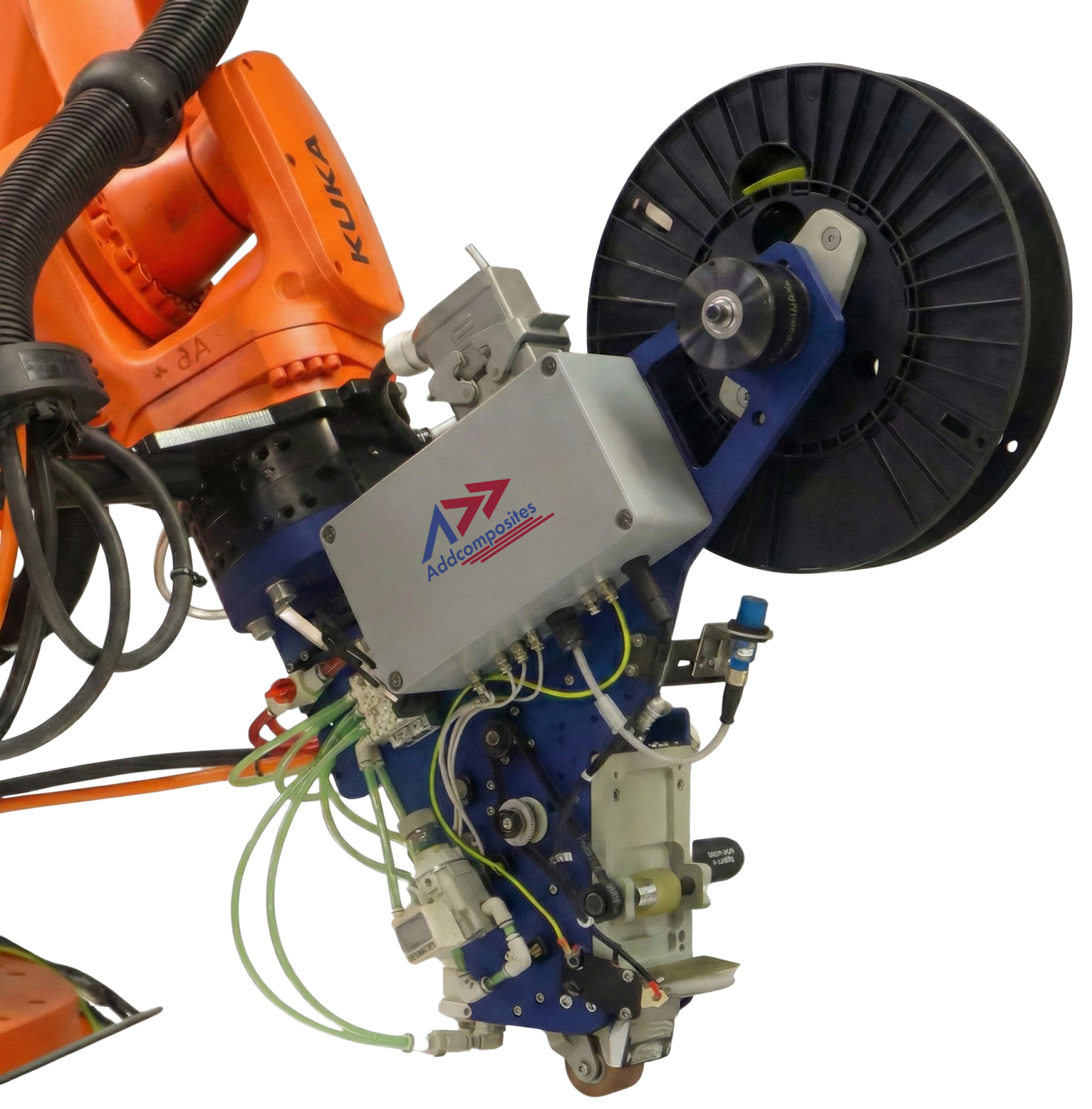
Multi-Axis Robotic Freedom

Compact AFP systems like the AFP-XS enable 6-DOF fiber placement on standard industrial robots. Multi-axis robotic systems possess the kinematic freedom to deposit material along arbitrary 3D paths. The question is no longer whether non-planar printing is mechanically possible, but rather: How do we generate toolpaths that exploit this freedom?

This review examines three interconnected algorithmic domains:

Non-Planar Slicing — Algorithms that generate curved layers conforming to part geometry
Stress-Field Aligned Toolpaths — Methods that derive fiber trajectories from FEA stress analysis
Geodesic and Steered Path Planning — The mathematics of keeping fibers from buckling or lifting on curved surfaces

THE LITERATURE GAP

While planar slicing algorithms for FDM are mature and well-documented, the literature on vector-field based slicing—algorithms that generate toolpaths based on FEA stress analysis rather than simple geometric intersection—remains fragmented. Most published work focuses on either non-planar geometry OR stress alignment, but rarely integrates both into a unified framework suitable for robotic continuous fiber printing.

The 2.5D Limitation

What is 2.5D Printing?

In conventional additive manufacturing, parts are "sliced" by intersecting the 3D model with a series of horizontal planes at fixed Z-heights. The resulting 2D contours define the toolpath for each layer. The Z-axis moves only between layers—never during material deposition.

This approach has three consequences for continuous fiber composites:

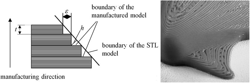
FIGURE 2: The Staircase Effect in 2.5D Printing

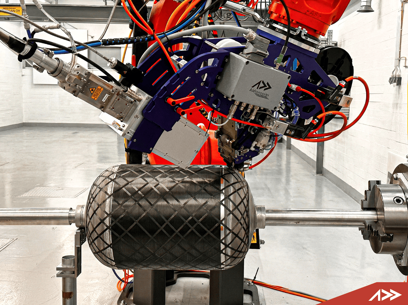
Conformal Deposition

AFP-XS depositing continuous fiber conformally on a curved surface, eliminating the staircase effect inherent in 2.5D approaches.

Slicing Strategy Comparison: Planar vs Non-Planar

How layer geometry impacts surface quality, fiber continuity, and structural performance

2.5D Planar Slicing

Surface roughness Ra > 10 μm

Layer height Fixed 0.2 mm

Fiber continuity Discontinuous

Stress concentrations At step edges

Non-Planar Slicing

Surface roughness Ra < 3 μm

Layer geometry Follows curvature

Fiber continuity Continuous

Stress concentrations Minimised

Concept based on Ahlers et al. (2019) — "3D Printing of Nonplanar Layers for Smooth Surface Generation" — IEEE CASE 2019

Consequence 1: The Staircase Effect

When a curved surface is approximated by planar layers, a "staircase" or "stair-stepping" artifact appears. For unfilled polymers, this is primarily an aesthetic and surface finish concern. For continuous fiber composites, it creates:

⚠️

Fiber discontinuities at layer transitions

⚠️

Stress concentrations at step edges

⚠️

Reduced interlaminar strength due to geometric notches

📊

Research by Ahlers et al. demonstrated that non-planar layers can reduce surface roughness by 63% compared to planar slicing

Consequence 2: Fiber Orientation Constraints

In 2.5D printing, fibers can only be oriented within the XY plane. They cannot:

Follow out-of-plane curvature (e.g., dome surfaces)
Align with 3D principal stress trajectories
Wrap continuously around convex geometries

This fundamentally limits the structural efficiency achievable through fiber placement.

Consequence 3: Support Requirements

Complex overhanging geometries require support structures in 2.5D printing. Multi-axis non-planar approaches can orient the deposition head normal to the local surface, eliminating the need for supports on many geometries that would otherwise be unprintable.

Non-Planar Slicing Fundamentals

Taxonomy of Non-Planar Approaches

Non-planar slicing algorithms can be categorized by their primary objective:

Approach	Primary Goal	Method	Key Papers
Surface-conforming	Eliminate staircase	Offset from top surface	Ahlers 2019, Chakraborty 2008
Iso-surface	Functional optimization	Scalar field iso-surfaces	Fang 2024, Liu 2024
Stress-aligned	Structural performance	FEA-driven vector fields	Fang 2024, Li 2022
Geodesic	Manufacturing feasibility	Shortest paths on surfaces	Diehl 2013, Sun 2020
Adaptive thickness	Material efficiency	Variable layer height	Allen 2020, Jin 2017

Non-Planar Slicing Strategies

Four approaches to generating curved-layer toolpaths for multi-axis deposition

Surface-Conforming

Layers are offset inward from the outer part surface

CAD-Driven Constant Offset Near-Net Shape

How It Works

The outermost layer conforms exactly to the CAD surface. Subsequent layers are generated by offsetting inward by a constant distance d (≈ layer height). Best for thin-walled parts where surface finish is critical. Requires collision checking for concave regions.

Iso-Surface (Thermal)

Layers follow virtual isothermal contours from FEA

FEA-Driven Thermal Field Process-Aware

How It Works

A thermal or scalar field is computed via FEA across the part volume. Layers are extracted as iso-surfaces of this field (e.g., T₁ > T₂ > T₃). This ensures each layer experiences uniform thermal history, reducing residual stress and warpage — especially valuable for semi-crystalline polymers like PEEK.

Stress-Aligned

Fiber paths follow first principal stress σ₁ directions

FEA → Streamlines Load-Optimised Max Efficiency

How It Works

FEA computes the principal stress tensor field. Fiber paths are generated as streamlines of σ₁ (first principal stress). This aligns every tow with the maximum tensile load direction, achieving up to 50% weight reduction vs. quasi-isotropic layups. Requires variable-angle steering capability.

Geodesic Paths

Shortest-distance trajectories along the part surface

Differential Geometry Min Steering Natural Fiber Paths

How It Works

Geodesic paths are the shortest curves between two points on a surface — the equivalent of "straight lines" in curved space. Fibers deposited along geodesics require minimal in-plane steering, preventing fiber wrinkling and maintaining consistent tow width. Ideal for doubly-curved geometries and winding patterns.

Part Surface

Toolpath / Fiber Path

Iso-Surface Contour

σ₁ Direction

Concept based on Liu et al. (2024) — "Neural Slicer for Multi-Axis 3D Printing" — ACM TOG 43(4)

The Collision Constraint

Any non-planar toolpath must be collision-free—the print head and robot arm must not intersect previously deposited material. This imposes geometric constraints that planar slicing trivially satisfies (always print from bottom to top) but non-planar slicing must explicitly solve.

QuickCurve (Etienne et al., 2024)

Addresses this through "slightly non-planar" surfaces that limit maximum deviation from horizontal, ensuring the nozzle always has clearance.

Neural Slicer (Liu et al., 2024)

Uses a learned neural network to optimize slicing surfaces while satisfying collision constraints through an energy-based formulation.

Iso-Surface Slicing Algorithms

The Isothermal Analogy

One elegant approach to generating curved slicing surfaces comes from thermal simulation. Proposed by Xu et al. (2022), the method works as follows:

Place the model virtually on a heated freeform substrate
Simulate heat conduction through the model
Extract isothermal surfaces (surfaces of constant temperature)
Use these isotherms as slicing layers

Isothermal Surface Slicing

Using steady-state thermal fields to generate naturally conformal non-planar layers

Benefits

✓

Natural conformity to heated substrate — layers curve organically following physics

✓

Smooth transitions between layers — no abrupt geometry changes

✓

Uniform thermal history per layer reduces residual stress and warpage

✓

Eliminates manual layer design — automatically derived from thermal FEA

Challenges

Tailoring thermal properties (k, h) for desired layer spacing requires iteration

Layer thickness varies with local geometry — thinner at convex, thicker at concave regions

Substrate heating infrastructure adds system complexity and energy cost

Requires multi-axis motion for nozzle to follow curved isothermal paths

Concept based on Xu et al. (2022) — "Additive manufacturing of non-planar layers using isothermal surface slicing" — J. Manuf. Proc. 84

The temperature field T(x,y,z) satisfies Laplace's equation:

∇²T = 0

By tailoring boundary conditions (base temperature, ambient temperature, surface convection) and assigning different thermal conductivities to regions of the model, the resulting isotherms can be shaped to achieve:

Conformal layers following the substrate
Variable layer thickness based on local geometry
Smooth transitions between regions

Reported improvements:

0 % decrease in surface roughness

0 % increase in tensile strength

0 % reduction in print time (certain geometries)

Scalar Field Optimization

More generally, non-planar layers can be generated by computing an optimal scalar field φ(x,y,z) and extracting its level sets (iso-surfaces) as slicing layers.

The design problem becomes: What scalar field produces iso-surfaces that satisfy our objectives?

Objectives may include:

Conforming to top surfaces (minimize staircase)
Aligning with stress directions in critical regions
Maintaining printable layer thickness
Avoiding collisions

Liu et al. (2024) formulate this as a differentiable optimization:

min_φ ℒ = λ₁ ℒ_surface + λ₂ ℒ_collision + λ₃ ℒ_thickness

Where:

ℒ_surface penalizes deviation from target surface
ℒ_collision penalizes print head collisions
ℒ_thickness maintains uniform layer thickness

Principal Stress-Aligned Toolpaths

The Structural Optimization Motivation

For continuous fiber composites, fiber orientation is not merely a manufacturing parameter—it determines structural performance. Aligning fibers with principal stress directions maximizes the utilization of the fiber's tensile properties.

Principal Stress Field (σ₁) — Plate with Central Hole

How tensile load redistributes around a discontinuity, and why fiber alignment matters

TRADITIONAL Raster Infill

3.0× stress concentration factor
Fibers cut at hole boundary. No load transfer around the discontinuity — stress concentrations remain at the theoretical maximum.

OPTIMISED Stress-Aligned

3.2× stress reduction (FEA verified)
Fibers wrap continuously around the hole following σ₁ streamlines. Load transfers smoothly — effectively eliminates the stress concentration.

Concept based on Sugiyama et al. (2022) — "Stress-adapted fiber orientation along the principal stress directions" — Prog. Addit. Manuf.

FEA-Driven Toolpath Generation

The general workflow for stress-aligned toolpath generation:

FEA-to-Toolpath Pipeline

From CAD model to stress-aligned deposition paths in five computational steps

Workflow applies to both 2.5D and non-planar toolpath generation for continuous fiber composites

The Vector Field Problem

The stress tensor at each point yields principal directions through eigenvalue decomposition:

σ_ij v_k = λ_k v_k

Where v₁ corresponds to the maximum principal stress direction (the optimal fiber alignment for tension-dominated loading).

Challenge: The vector field formed by v₁ directions is typically:

🔀

Not smooth — Discontinuities at material boundaries

📐

Not divergence-free — Streamlines may converge/diverge

⚡

Singular — Undefined at isotropic stress states where σ₁ = σ₂

Field-Based Toolpath Methods

Li et al. (2022) proposed a field-based toolpath generation approach that addresses these challenges:

Harmonic field smoothing — Project the stress directions onto a smooth vector field
Stream surface generation — Create surfaces whose tangent aligns with the smoothed field
Iso-curve extraction — Extract toolpaths as curves on the stream surfaces

Digital Twin to Physical Part

From digital twin to physical part: AddPath simulation and corresponding AFP-XS deposition.

From Stress Field to Toolpaths

Four-stage pipeline: stress tensor → smoothed vector field → streamlines → printable fiber paths

Raw Stress Field

Noisy, singular points present

Smoothed Vector Field

Smooth, integrable field

Streamline Integration

Tangent to v₁ — principal direction

Final Toolpaths

Spaced for fiber tow width — print-ready

Source: Li et al. (2022), "Field-Based Toolpath Generation for 3D Printing Continuous Fibre Reinforced Thermoplastic Composites," Additive Manufacturing, 49.

Principal Stress Lines (PSL)

An alternative approach extracts Principal Stress Lines directly from the stress field—curves that are everywhere tangent to a principal stress direction.

Fang et al. (2024) demonstrated that PSL-based toolpaths achieve significantly higher fiber coverage in regions of stress concentration compared to raster patterns:

Method	Fiber Coverage	Load Capacity vs. XY-Planar
XY-planar raster	~65%	1.0× (baseline)
Principal stress lines	~90%	6.35×
Stress-aligned iso-surfaces	~85%	4.5× (5-DOF system)

The key finding: stress-aligned toolpaths in critical regions dramatically improve structural performance, with reported load capacity improvements of 4-6× compared to conventional planar approaches.

Geodesic vs. Steered Fiber Paths

The Path Geometry Problem

When depositing continuous fiber on a curved surface, the fiber path must satisfy geometric constraints to avoid defects. Two fundamental path types exist:

Geodesic Paths

The shortest path between two points on a surface (zero geodesic curvature)

Steered Paths

Paths that deviate from geodesics to achieve desired fiber orientation

Geodesic vs. Steered Paths on Curved Surfaces

Comparing zero geodesic curvature (κ_g = 0) and variable-angle steering (κ_g ≠ 0) strategies for AFP

Manufacturing Comparison

Property	Geodesic (κ_g = 0)	Steered (κ_g ≠ 0)
Fiber Tension	Uniform along path Stable	Variable — higher at inner radius Monitor
Slippage Risk	Low — natural adherence Low	High — lateral force on tow High
Wrinkling Risk	None — zero in-plane curvature None	Possible — inner-edge compression Risk
Orientation Control	Limited — geometry-dictated Fixed	Full — any angle achievable Flexible
Path Coverage	Natural spacing — may diverge Gaps	Controllable — gaps/overlaps tunable Tunable

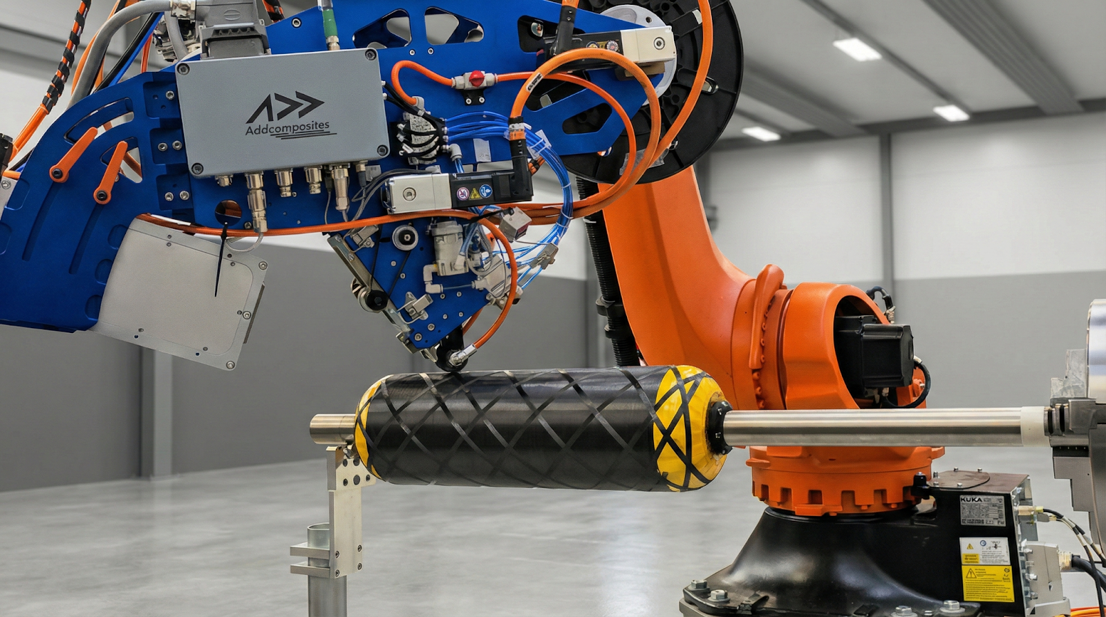
Concept based on Shirinzadeh et al. (2019) — "Automated Fiber Placement Path Planning: A state-of-the-art review" — CAD J. 16(2)

Geodesic Fiber Placement

AFP-XS performing geodesic fiber placement on a cylindrical mandrel, demonstrating the system's multi-axis path following capability.

Mathematical Framework

On a curved surface, a path γ(s) parameterized by arc length has two curvature components:

Normal curvature (κ_n) Curvature in the direction normal to the surface (determined by surface geometry)

Geodesic curvature (κ_g) Curvature within the tangent plane (controllable through path design)

A geodesic is a path with κ_g = 0. For fiber placement:

Total curvature: κ = √(κ_n² + κ_g²)

The fiber experiences lateral forces proportional to geodesic curvature. When κ_g exceeds a threshold, the fiber will buckle/wrinkle on the inside of the curve (compression) or lift/slip on the outside of the curve (tension).

Steering Radius Limits

The minimum steering radius R_min defines the tightest curve a fiber tow can follow without defects:

R_min = 1 / κ_g,max

Typical values for carbon fiber prepreg:

Tow Width	Material	Min Steering Radius	Source
6.35 mm (1/4")	CF/Epoxy	500-700 mm	Industry standard
3.175 mm (1/8")	CF/PEEK	300-400 mm	Lukaszewicz 2012
6.35 mm (1/4")	CF/PEKK	400-600 mm	Experimental

The minimum steering radius depends on tow width (wider = larger radius required), matrix tack (lower tack = more slippage), substrate curvature (affects normal forces), compaction pressure (higher = better adhesion), and deposition temperature (affects matrix flow).

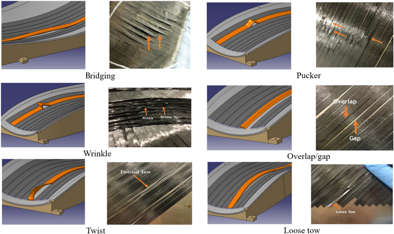
FIGURE 8: Steering Defects in Variable Angle Tow Placement

Defects from Excessive Steering

Three primary manufacturing defects in variable-angle AFP when geodesic curvature exceeds process limits

A Tow Wrinkling

κ_g > κ_g,max

Inner edge compresses, outer edge stretches — when curvature exceeds the critical radius, the inner edge buckles out-of-plane.

Mechanism & Limits

For a 6.35 mm (¼") tow, minimum steering radius is typically 600–800 mm. Below this, the inner-edge compressive strain exceeds the matrix yield strain, causing sinusoidal buckling (wrinkling). Severity increases with tow width and ply thickness. Detection requires visual inspection or profilometry.

B Gap Formation

Tow-drop method — coverage deficit

When tows are dropped at ply boundaries to avoid overlap, uncovered regions form resin-rich pockets with no fiber reinforcement.

Mechanism & Impact

The tow-drop method terminates individual tows at a ply boundary to maintain uniform thickness, but leaves gaps (Δ) between courses. These resin-rich regions act as crack initiation sites and reduce the effective fiber volume fraction locally. Gaps wider than 2 mm significantly affect compression-after-impact performance.

C Overlap Formation

Adjacent tow edges encroach

Tow edges encroach on adjacent courses, creating local thickness buildup and fiber waviness at the overlap boundary.

Mechanism & Impact

Overlaps add an extra tow thickness (+t ≈ 0.15–0.25 mm) locally. This creates surface height steps that propagate through subsequent plies, causing fiber waviness, resin pockets at overlap edges, and local stress concentrations up to 1.5× nominal. They also compromise aerodynamic surface quality.

Impact on Structural Performance

📉

~15%

Buckling load reduction
(from gaps)

LowSeverityHigh

⚡

1.5×

Local stress concentration
(from overlaps)

LowSeverityHigh

🔄

↓↓

Reduced fatigue life
(both gaps & overlaps)

LowSeverityHigh

Concept based on Heinecke & Willberg (2019) — "Manufacturing-Induced Imperfections in Composite Parts Manufactured via AFP" — J. Compos. Sci. 3(2)

Variable Angle Tow (VAT) Laminates

Variable Angle Tow composites intentionally use steered fiber paths to tailor stiffness distribution. The fiber angle varies continuously across the laminate, typically described by:

θ(x) = θ₀ + (θ₁ − θ₀) / L × x

Where θ₀ is the angle at the center and θ₁ is the angle at the edge, over half-width L.

Benefits of VAT:

Improved buckling resistance (up to 80% higher critical load)
Tailored load paths around cutouts
Reduced stress concentrations
Optimized stiffness-to-weight ratio

Manufacturing challenges:

Gaps and overlaps at path boundaries
Thickness variation
Process parameter optimization
Requires steering within R_min limits

Continuous Tow Shearing (CTS)

An alternative to traditional AFP steering, Continuous Tow Shearing (CTS) uses the ability to shear dry fiber tows rather than bend them:

Continuous Tow Shearing (CTS) vs. Conventional AFP Steering

Fiber steering mechanism comparison for variable angle tow composites

Conventional AFP

In-Plane Bending

Inner edge: Compression → fiber buckling

Outer edge: Tension → gaps & tow pull

Result: Wrinkling limits steering radius

~500 mm

Minimum Steering Radius

For 6.35 mm (¼") tow width

Continuous Tow Shearing

Shear Deformation

Mechanism: Fibers shear, not bend

Stress: No in-plane compression or tension

Result: Tighter radii, no wrinkling defects

~50–100 mm

Minimum Steering Radius

Depending on shear angle limit

Source: Beakou et al. (2014), "Manufacturing characteristics of the continuous tow shearing method," Composites Part A, 66.

CTS Advantages

Significantly tighter steering radii (5-10× improvement)
Reduced process-induced defects
Better fiber alignment with designed orientation

CTS Limitations

Currently limited to dry fiber (subsequent infusion required)
Shear strain limits exist (typically < 30°)
Equipment more complex than standard AFP

Manufacturing Constraints

Multi-Axis Robot Kinematics

6-DOF industrial robots provide the kinematic freedom for non-planar printing, but introduce constraints:

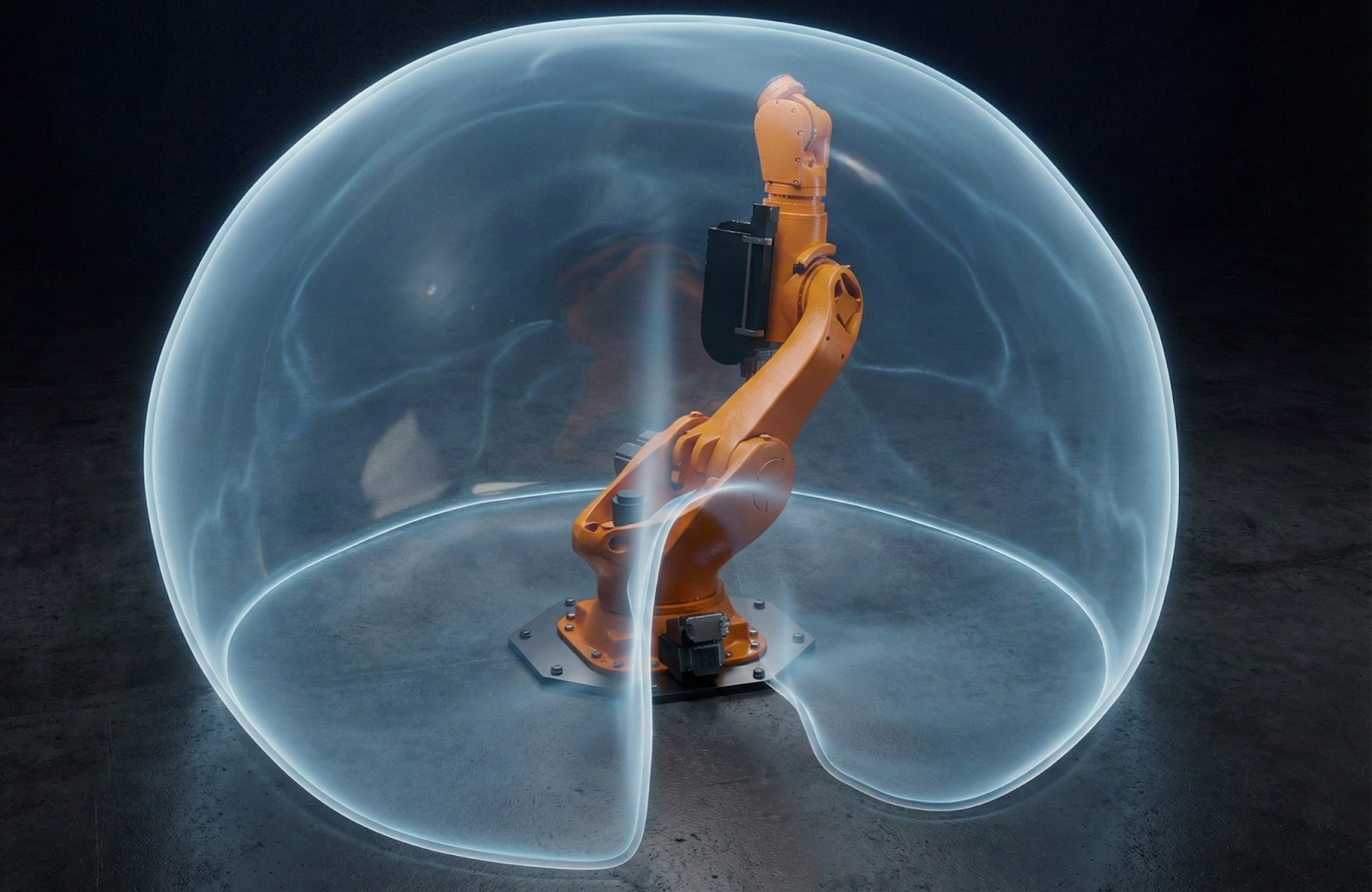
Robot Workspace Constraints

FIGURE 10: Robot Workspace and Singularity Constraints. The reachable workspace, joint limits, singularities, and collision boundaries all constrain the toolpath planning envelope.

6-DOF Robot Considerations for Non-Planar Printing

Workspace, kinematic constraints & toolpath requirements for robotic AFP/LFAM

Reachable Workspace Envelope

Kinematic Constraints

Joint Limits

Each axis has ±θ_max rotational bounds

→ Limits reachable orientations at workspace edges

Singularities

Wrist singularity at extended reach positions

→ Infinite joint velocities near singular configs

Collision Avoidance

Self-collision & environment collision checks

→ Real-time swept volume monitoring required

Velocity Limits

Max joint speeds constrain TCP velocity

→ Non-uniform deposition if TCP speed varies

Acceleration Limits

Dynamic limits for smooth motion profiles

→ Critical for fiber tension & compaction control

Toolpath Requirements for Non-Planar Deposition

Continuous Orientation

Smooth orientation changes along path — avoid wrist flip discontinuities

Reachable Envelope

Entire part must fit within the robot's feasible workspace

Constant TCP Velocity

Uniform speed at tool center point for consistent material deposition

Smooth Acceleration

Jerk-limited profiles for fiber tension and compaction force control

Process Parameter Interdependencies

Non-planar continuous fiber printing involves coupled parameters:

Parameter	Planar Printing	Non-Planar Complexity
Layer height	Constant	Varies with surface normal
Deposition rate	Constant	Varies with curvature
Compaction force	Normal to bed	Normal to local surface
Temperature	Uniform	Varies with head orientation
Robot speed	2-DOF (XY)	6-DOF, joint-limited

Collision Detection

Non-planar toolpaths require explicit collision checking:

🔧

Nozzle-to-part collision — The print head must not hit already-printed material

🤖

Robot-to-part collision — Robot links must clear the part

🏭

Robot-to-environment collision — Fixtures, enclosure, etc.

Modern slicers address this through configuration space analysis (C-space obstacles), signed distance fields for fast collision queries, and incremental collision checking along toolpath.

Performance Improvements

Structural Performance Gains

Published studies report dramatic improvements from stress-aligned and non-planar toolpaths:

Mechanical Performance: Stress-Aligned vs. Conventional

Load capacity and stress concentration improvements through optimized fiber orientation

Load Capacity Comparison

Normalized to XY-Planar baseline = 1.0×

XY-Planar
(baseline)

1.0×

Stress-Aligned
2D, in-plane

2.3×

Stress-Aligned
5-DOF, hemispherical

4.5×

Iso-Surface Aligned
multi-axis

6.35×

Peak improvement over baseline: 6.35× load capacity

Stress Reduction at Notch / Hole

Stress concentration factor comparison

Straight Fiber
0°/90° layup

3.0×

Stress-Adapted
optimized orientation

0.94×

3.0×

Straight Fiber SCF

→

0.94×

Stress-Adapted SCF

→

3.2×

Stress Reduction

Sources: Fang et al. (2024), arXiv:2410.16851; Sugiyama et al. (2022), Progress in Additive Manufacturing.

Key Performance Data

Study	Method	Test Case	Improvement
Fang 2024	PSL + iso-surfaces	Tensile specimens	6.35× load capacity
Fang 2024	5-DOF stress-aligned	Hemispherical caps	4.5× burst pressure
Sugiyama 2022	Stress-adapted	Plate with hole	3.2× stress reduction
Matsuzaki 2016	Curved layer FDM	Beam bending	25% stiffness increase
Li 2022	Field-based	Bracket	90% fiber coverage

Surface Quality Improvements

Non-planar slicing also improves surface finish:

Method	Surface Roughness (Ra)	Improvement vs. Planar
2.5D planar (0.2mm layer)	10-15 μm	Baseline
Surface-conforming	3-5 μm	63% reduction
Adaptive thickness	5-8 μm	40% reduction
Isothermal surfaces	4-6 μm	55% reduction

Computational Methods

Topology Optimization Integration

The most advanced approaches integrate toolpath generation with topology optimization:

Integrated Topology and Toolpath Optimization

Simultaneous material layout & fiber path optimization for layer-free multi-axis AM

Design Inputs

Design domain

Load cases & boundary conditions

Manufacturing constraints (min radius, fiber width)

Simultaneous Optimization Loop

Topology Optimization

obj Minimize compliance

var ρ(x, y, z) — density field

out Optimized material layout (geometry)

Toolpath Optimization

obj Minimize stress deviation

var φ(x, y, z) — scalar field for iso-surface extraction

out Stress-aligned fiber paths on iso-surfaces

Outputs

Optimized Geometry

Topology-optimized shape with minimum compliance

ρ(x,y,z) → solid/void boundaries

Optimized Fiber Paths

Stress-aligned orientations on iso-surfaces

φ(x,y,z) → principal stress alignment

Printable Toolpath

Collision-free multi-axis deposition path

Robot-ready G-code / waypoints

Source: Zhou et al. (2025), "Simultaneous Topology and Toolpath Optimization for Layer-Free Multi-Axis Additive Manufacturing," Additive Manufacturing.

Algorithm Complexity

Algorithm Component	Complexity	Typical Runtime
FEA solve	O(n³)	Seconds to minutes
Eigenvector decomposition	O(n) per element	Fast
Vector field smoothing	O(n log n)	Seconds
Streamline integration	O(m × n)	Seconds
Collision detection	O(p × log n)	Per-point check
Toolpath optimization	Iterative	Minutes to hours

Where n = mesh elements, m = number of streamlines, p = toolpath points.

AddPath Platform

AddPath: integrated path planning, simulation, and robot code generation for automated fiber placement — from design to manufacturing in a single environment.

Software Tools

Tool	Type	Non-Planar Support	Stress Alignment
Cura	Open-source	Plugin (limited)	No
PrusaSlicer	Open-source	No	No
S4-Slicer	Research	Yes	No
FullControl	Python library	Yes	Research
ADDCOMPOSITES	Commercial	Yes	Yes
Ansys ACP	Commercial	Yes	FEA integration

Industrial Applications

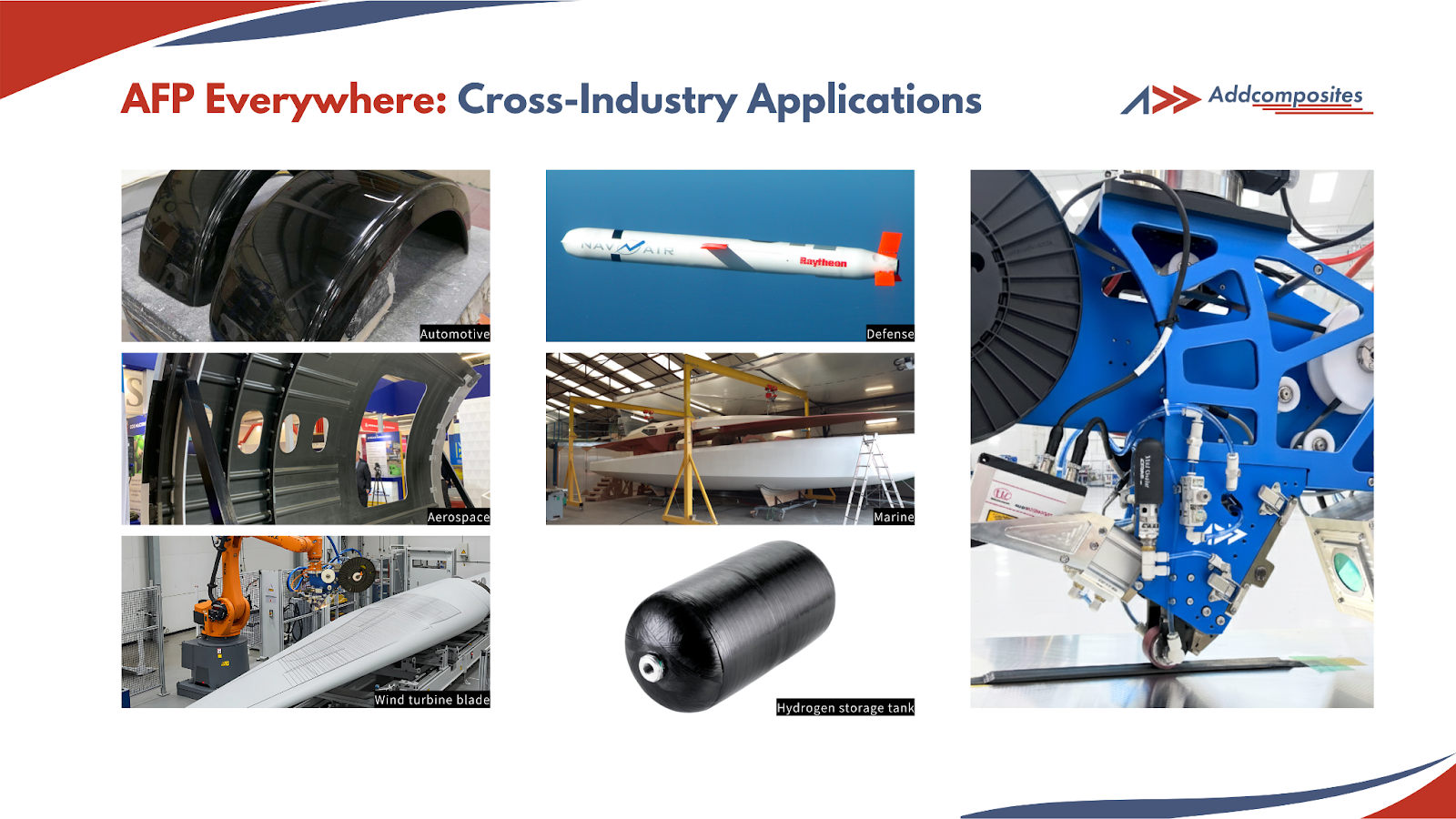
FIGURE 13: Aerospace Application Examples

Aerospace Applications — Non-Planar Continuous Fiber

Structural performance gains through stress-aligned, multi-axis fiber deposition

Pressure Vessel / Dome

Helical fiber winding paths follow geodesic trajectories on dome surfaces, aligning fibers with principal hoop and meridional stresses for maximum burst resistance.

4.5×

Burst Pressure vs. Planar

Propellant tanks

Load-Carrying Panel with Cutout

Continuous fibers are steered around structural cutouts, following principal stress trajectories to minimize stress concentration at hole boundaries.

3× Reduced

Stress Concentration

Fuselage panels & wing skins

Conformal Tooling

Non-planar deposition conforms fiber layers directly to curved mold surfaces, eliminating inter-layer stepping artifacts and achieving near-net-shape surface accuracy.

<0.1 mm

Surface Accuracy

Composite tooling & mandrels

Current Industrial Implementations

Company	Application	Technology	Status
9T Labs	Structural brackets	Stress-optimized, planar	Production
Arevo	Bike frames	Multi-axis, non-planar	Production
Continuous Composites	Large structures	7-axis robot	Development
CEAD	Large-scale AM	Gantry, non-planar capable	Production
AddComposites	Research systems	AFP robot integration	Commercial

Future Directions

Near-Term Developments (2025-2028)

Unified slicing frameworks integrating non-planar geometry, stress alignment, and collision avoidance
Real-time adaptive toolpaths responding to in-situ process monitoring
Multi-material non-planar printing with strategic material placement
Standardization of non-planar toolpath formats (beyond G-code)

Medium-Term Research (2028-2032)

AI-driven toolpath optimization — Neural networks trained on FEA data predicting optimal paths
Closed-loop stress-adaptive printing — Real-time FEA updates during printing
Hybrid manufacturing — Integration with CNC machining for final surfaces
Certification pathways — Qualification methods for non-planar printed primary structure

Open Research Questions

How to handle multi-load case optimization when stress fields differ?
What are the fatigue implications of stress-aligned vs. traditional laminates?
Can machine learning predict steering defects before they occur?
How to certify parts with spatially varying fiber orientation?

Conclusions

Summary of Key Findings

The 2.5D constraint is no longer necessary. Multi-axis robots provide kinematic freedom for true 3D toolpaths, and algorithms exist to exploit this freedom.

Non-planar slicing reduces surface roughness by 50-65% and eliminates the staircase effect on curved geometries.

Stress-aligned toolpaths improve structural performance by 3-6× compared to conventional raster patterns, particularly in regions of stress concentration.

Geodesic paths are manufacturing-safe but orientation-limited. Steered paths offer orientation control but require careful attention to steering radius limits.

Integrated topology and toolpath optimization represents the frontier, simultaneously optimizing what to print and how to print it.

Manufacturing constraints remain critical. Minimum steering radius, collision avoidance, and robot kinematics constrain the theoretical optimum.

Practical Guidance

For engineers considering stress-aligned non-planar printing:

Application	Recommended Approach	Key Constraints
Pressure vessels	Geodesic + slight steering	Fiber continuity
Panels with holes	PSL-aligned	Steering radius at concentration
Complex 3D surfaces	Iso-surface + field-based	Collision, robot reach
Production parts	Start with planar VAT	Manufacturing maturity
R&D/prototypes	Full non-planar, stress-aligned	Compute time

The Bigger Picture

Non-planar slicing and stress-aligned toolpaths represent a fundamental shift in how we think about additive manufacturing. Rather than asking "how do we manufacture this shape?" we can now ask "what shape and fiber arrangement optimally carries these loads?"

For continuous fiber composites, this is transformative. The anisotropy that makes composites challenging to design with becomes an opportunity when fiber placement can be optimized in three dimensions.

The technology readiness is advancing rapidly. Within the next 5 years, stress-aligned non-planar printing will likely transition from research demonstrations to production applications, first in aerospace (where performance justifies cost) and eventually in automotive and industrial applications.

The limiting factor is no longer the robot or the material—it's the algorithms and software that bridge the gap between structural design and manufacturing execution.

References

[1] Ahlers, D., Wasserfall, F., Hendrich, N., Zhang, J. (2019). 3D Printing of Nonplanar Layers for Smooth Surface Generation. IEEE CASE 2019. DOI

[2] Fang, G., et al. (2024). Toolpath Generation for High Density Spatial Fiber Printing Guided by Principal Stresses. arXiv:2410.16851

[3] Fang, G., et al. (2024). Exceptional mechanical performance by spatial printing with continuous fiber: Curved slicing, toolpath generation and physical verification. Additive Manufacturing, 82, 104048.

[4] Liu, H., et al. (2024). Neural Slicer for Multi-Axis 3D Printing. ACM Transactions on Graphics, 43(4). DOI

[5] Li, B., et al. (2022). Field-Based Toolpath Generation for 3D Printing Continuous Fibre Reinforced Thermoplastic Composites. Additive Manufacturing, 49, 102467. DOI

[6] Xu, J., et al. (2022). Additive manufacturing of non-planar layers using isothermal surface slicing. Journal of Manufacturing Processes, 84. DOI

[7] Etienne, J., et al. (2024). QuickCurve: Revisiting slightly non-planar 3D printing. arXiv:2406.03966

[8] Sugiyama, K., et al. (2022). Stress-adapted fiber orientation along the principal stress directions for continuous fiber-reinforced material extrusion. Progress in Additive Manufacturing. DOI

[9] Shirinzadeh, B., et al. (2019). Automated Fiber Placement Path Planning: A state-of-the-art review. Computer-Aided Design and Applications, 16(2), 172-203.

[10] Beakou, A., et al. (2014). Manufacturing characteristics of the continuous tow shearing method for manufacturing of variable angle tow composites. Composites Part A, 66. DOI

[11] Heinecke, F., Willberg, C. (2019). Manufacturing-Induced Imperfections in Composite Parts Manufactured via Automated Fiber Placement. Journal of Composites Science, 3(2). DOI

[12] Allen, R., Trask, R. (2020). Additive manufacturing of non-planar layers with variable layer height. Additive Manufacturing, 36, 101556.

[13] Jin, Y., et al. (2017). Variable-depth curved layer fused deposition modeling of thin-shells. Robotics and Computer-Integrated Manufacturing, 48, 25-35.

[14] Lukaszewicz, D.H.J.A., et al. (2012). The engineering aspects of automated prepreg layup: History, present and future. Composites Part B, 43(3), 997-1009.

[15] Zhou, Y., et al. (2025). Simultaneous Topology and Toolpath Optimization for Layer-Free Multi-Axis Additive Manufacturing of 3D Composite Structures. Additive Manufacturing. DOI

[16] Fernandez, F., et al. (2025). Non-planar 3D printing: Enhancing design potentials by advanced slicing algorithms and path planning. Procedia CIRP.

[17] Wang, Z., et al. (2024). A fully automatic non-planar slicing algorithm for the additive manufacturing of complex geometries. Additive Manufacturing, 71, 103583. DOI

[18] Diehl, T., et al. (2013). Function-aware slicing using principal stress line for toolpath planning in additive manufacturing. Journal of Manufacturing Science and Engineering.

[19] Sun, Z., et al. (2020). An efficient pre-analysis and optimization generation method for reference curves of automated fiber placement path planning. Journal of Composite Materials. DOI

[20] CompositesWorld (2024). Automated fiber placement: The evolution from industrial to accessible.

This article was compiled using the Research-to-Publication pipeline, synthesizing findings from peer-reviewed academic publications and industry sources. The review focuses on algorithmic and computational aspects of non-planar continuous fiber printing.

Last updated: January 2025

Learn More

AFP-XS Entry-level automated fiber placement

AFP-X Advanced multi-tow system

AddPath AI-powered path planning software

Complete Guide The Complete Guide to AFP Machines

Have questions about implementing non-planar slicing and stress-aligned toolpaths for your composite manufacturing?

Pravin Luthada

CEO & Co-founder, Addcomposites

About Author

As the author of the Addcomposites blog, Pravin Luthada's insights are forged from a distinguished career in advanced materials, beginning as a space scientist at the Indian Space Research Organisation (ISRO). During his tenure, he gained hands-on expertise in manufacturing composite components for satellites and launch vehicles, where he witnessed firsthand the prohibitive costs of traditional Automated Fiber Placement (AFP) systems. This experience became the driving force behind his entrepreneurial venture, Addcomposites Oy, which he co-founded and now leads as CEO. The company is dedicated to democratizing advanced manufacturing by developing patented, plug-and-play AFP toolheads that make automation accessible and affordable. This unique journey from designing space-grade hardware to leading a disruptive technology company provides Pravin with a comprehensive, real-world perspective that informs his writing on the future of the composites industry.